Monday, November 26, 2012

Lab 8 - Station Fire


      The climatic conditions of the Southwestern United States are that of a desert- dry land, arid atmosphere, and overall minimal precipitation. Southern California, in particular, primarily has a Mediterranean climate, which means that it is cold and wet in the winter, but the summers are very hot and dry, and the vegetation is dominantly Chaparral. The dry summer climate and Chaparral that can easily withstand the dry conditions both contribute to the many fires that start in the Southern California region each year (World Wildlife Fund). This past August, the peak of the hot season, firefighters faced a blaze that was so difficult to handle, with the Station fire, that federal lands had to be sacrificed in order to protect human life and possessions.
     Although the cause of the fire was arson, according to the LA Times online newspaper, the climatic conditions of the region supported the fire's growth, and made it terribly difficult to contain. "On Tuesday, the backfire, or controlled burn, was canceled because of heavy winds, temperatures in the low 90s and relative humidity around 10%" (Lopez). Also, while firefighters desperately tried to contain the flames from spreading "the fire....sent plumes of thick smoke spiraling as much as 20,000 feet into the air....creating its own wind patterns, [and] making it unpredictable" (Marciano). Overall, the weather conditions in fact made it worse for the firefighters to complete their task.
     Due to the Chaparral's ability to burn easily, and the build up of the vegetation from decades of no fires burning in that specific area, the Station fire had plenty of fuel to not only last, but to grow immensely in a very short time span. "Efforts [by the firefighters] have been impeded by the extremely difficult terrain, vegetation that has not burned for over four decades and hot and dry weather conditions" (AHN). Refer to the map of the distribution of vegetation in Los Angeles County; this map shows the geographical relationship between the spread of the Station fire from August 29 to September 2 and the location of vegetation in that area. Notice that there is a significant amount of vegetation to the north and east of the origion of the fire, while, in contrast, there is very little vegetation to the south. The spread of the fire follows the path presented by the vegetation, and travels due north and east during its initial spread.
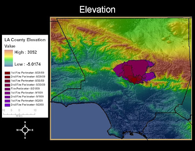
     The firefighters main concern while combatting the flames were to protect the neighboring population and keep major highways open by prioritizing the containment of the fire on the south and west ends. According to the LA Times "Most of the fire's growth Thursday took shape on its eastern flank", and "on thursday, around noon, officials closed southern part of the Angeles National Forest" (Blankstein). Even though the Angeles National Forest is located to the north of the origin of the fire, officials were determined to deter the fire from the population and sacrifice the national forest, which is on federal lands. Notice on the "Private vs Public Land" map the spatial relationship between the private land held by the population and public land that belongs to the government, and both of their relationships to the spread of the fire. As the map shows, over time the fire grew away from private lands, represented by the pink shade, and overtook parts of property that is owned by the government, represented by the yellow shade.
     Althought the weather conditions, vegetation, and terrain made it difficult for the fire fighters to contain all perimeters of the fire, the heros did receive some help from unsuspecting sources in detering the flames away from private property. While the vegetation fueled the fire's great spread, it also pulled the fire to the north and east, away from the population. Also, "most of the fire's growth Thursday took shape on its eastern flank....where firefighters battling the blaze faced treacherous conditions, including steep terrain and rolling rocks (Blankstein). The terrain that made it so demanding to contain the flames was mainly located on the eastern side of the original fire, which fortunately was also away from residential areas and major roads.

References

AHN. "Update: Angeles National Forest Fire Now Over 140,000 Acres; Emergency Declared In San Bernardino County." Inquisitr September 2, 2009. Web. 24 Nov 2009. http://www.inquisitr.com/35595/update-angeles-national-forest-fire-now-over-140000-acres-emergency-declared-in-san-bernardino-county/.

Blankstein, Andrew; Bloomekatz, Ari; and DiMassa, Cara. "Station fire an act of arson, sheriff's officials say." Los Angeles Time (September 4, 2009): n. pag. Web. 24 Nov 2009. http://articles.latimes.com/2009/sep/04/local/me-fire4?pg=2.

Lopez, Robert and Winton, Richard . "Containment of Station fire slows amid unfavorable conditions." Los Angeles Time/ Local (September 9, 2009): n. pag. Web. 24 Nov 2009. http://latimesblogs.latimes.com/lanow/2009/09/containment-station-fire-slows.html.

Marciano, Rob, Chad Myers, John Torigoe, and Stephanie Chen. "Angry fire' roars across 100,000 California acres." CNN.com/US (August 31, 2009): n. pag. Web. 24 Nov 2009. http://www.cnn.com/2009/US/08/31/california.wildfires/index.html#cnnSTCPhoto.

World Wildlife Fund, . "California Chaparral and Woodlands." Wild World Ecoregion Profile. 2001. National Geographic, Web. 24 Nov 2009. http://www.worldwildlife.org/wildworld/profiles/g200/g121.html.

Wednesday, November 7, 2012

Lab 6 - DEM Analysts


The area I selected is located in the mountainous terrain of northern California. The upper boundary of the area is 41.34 decimal degrees north latitude, and the lower boundary is 40.83 decimal degrees north latitude. The left boundary of the area is -123.64 decimal degrees west longitude, and the right boundary is at -122.90 west longitude. The GCS is set on the North American Datum 1983.

Sunday, November 4, 2012

Lab 5 - Projections


Having different map projections available is very significant because each projection shows a different type of view of an area. For example, equidistant map projections preserve distance proportions between longitudinal lines. So the vertical distance on the map is proportional to its counterpart on the ground. Also, an equal area map preserves the area of the entities represented in the map. Then there is a conformal map projection, which preserves angles. Without all three types of projections a person looking at a map will always have to adjust their direction according to margin of error produced by the projection. However, with the many different types of map projections, people are able to choose that map that best fits for the purpose it is being used for. Even though the map projections are useful in helping us understand the world spatially, there is also a problem that arises when attempting to read a map.

The reason different map projections are even needed is because they all give some sort of misrepresentation of the world. This problem comes from stretching a spherical figure on to a planar surface. That translation between shapes creates the phenomenon in which there are different levels of distortion shown on each map projection. In general, the central focus area of each map is the most accurate, and as the map moves away from the center the distortions increase. While the various map projections have different types of distortion, they all follow the same pattern where there are varying levels of distortion within the same map.

There is great potential for the advancement in mapping itself. As technology continues to become more advanced, map projection gains more potential to deliver more accurate and precise representations of the world. For example, in the gis map projection lab assignment, six different types of maps were used- for equidistant maps I used Conic and Plate Carree, for equal area maps I used Mollweide and Goode Homolosine, and for conformal maps I used Mercator and Stereographic- and every map gave a different measurement for the distance between two consistent points. A feature that is presented in ArcMaps is a Geographic Coordinate System, which allows the user to view a representation of the world that is based on a 3D spherical shape so it is not planar like the map projections. In the future, it is possible that there may be portable maps that are able to use the same 3D feature as on computers.

However, due to the unavoidable phenomenon of distorting a spherical image when trying to translate it to a planar surface, map projections will never be perfect. When using a paper map, the distortions in size, shape, and angles must be accounted for in order to have correct guidance from the map. Therefore, having knowledge of the different types of map projections, their inaccuracies, and levels of distortion will prove to be very helpful, and make using a map to navigate through any part of the world at least a little easier.

Sunday, October 14, 2012

Lab 3 - Neogeography


View Pac 12 Universities in a larger map

Pitfalls, Potential, and Consequences of Neogeography

Neogeography is an interesting phenomena that resulted from the advancements in technology, and people's growing interest in social networking. Neogeography is an attractive concept to many because it is user-centric. It allows the user to create (or recreate) their own world using geographic information systems. In this world, the user is in control. The mapping of any and everything of value- places, things, memories, etc- in that world is at the user's discretion to decide. The user decides this by mapping whatever he or she likes. Due to the ease of Neogeographical tools and systems, it will most likely earn a greater interest among the technologically inclined, which in itself is growing with time.

Neogeography is a great way for people to express themselves or share, but because it is user centric and is open to anyone with computer access, the information displayed within the neogeography is more susceptible to falsehoods- whether intentional or accidental. When this information is displayed to others on the web, or by any other means, it must be viewed only as an insight into another person's newly created world.

Lab 2 - Beverley Hills Quadrangle

Lab 2 - Beverly Hill Quadrangle

1.) Name of Quadrangle
- Beverly Hills

2.) Names of Adjacent Quadrangles
- Canoga Park (NW),
- Van Nuys (N),
- Burbank (NE),
- Topanga (W),
- Hollywood (E),
- Venice (S)
- Inglewood (SE)

3.) Quadrangle (Map) First Created
- 1966

4.) Datum
- North American Datum of 1983 (NAD83)

5.) Scale
- 1 : 24,000

6.) Conversions Using Scale 1,200 meters 1.89 miles 2.64" 12.5 cm

7.) Contour Interval
- 20 feet

8.) Geographic Coordinates

a.) Public Affairs Building
- D/M/S: N Lat 34 degrees 4' 28" , W Lon: 118 degrees 26' 21"
- Decimal: N Lat 34.075 degrees , W Lon: 118.44 degrees

b.) tip of Santa Monica Pier
- D/M/S: N Lat 34 degree 0' 27" , W Lon 118 degrees 30' 0"
- Decimal: N Lat 34.01 degrees , W Lon 118.5 degrees

c.) top of Upper Franklin Canyon Resivoir
- D/M/S: N Lat 34 degrees 7' 23" , W Lon 118 degrees 27' 20"
- Decimal: N Lat 34.12 degrees , W Lon 118.46 degrees

9.) Elevation
elevation2

a.) Greystone Mansion (in Greystone Park)
- 495 feet
- 150.86 meters

b.) Woodlawn Cemetary
- 140 feet
- 42.67 meters

c.) Crestwood Hills park
- 660 feet
- m= 201.12 meters

10.) UTM Zone
- Zone 11

11.) UTM Coordinates
- 61 333m E , 62 975m N

12.) Number of square meters in a cell
- 1,000,000 m in one cell

13.) Elevation Across 73 71 000 Northin


14.) Magnetic Declination
- 14degrees East

15.) Direction of stream flow between 405 Freeway and Stone Canyon Reservoir
- southward flow

16.) Map of UCLA
UCAL in Beverly Hills Quadrangle

Monday, October 1, 2012

Lab 1 - 3 Interesting Maps - Jason Ward


This map displays the locations of sea ice features within the Antarctic Region. It is provided by Kevin Arrigo, a researcher at Standford University (Arrigo 2003). The map was created from SSM/I satellite imagery (Arrigo 2003). It displays 37 areas of open water imbedded within the contiguous ice cover about the Antarctic continent (Arrigo 2003). As soon from the legend provided with the map, areas of complete ice cover year-round are indicated by the red coloring. The areas that are completely devoid of ice cover all year are indicated by purple coloring. The intermediate colors on the legend (orange, yellow, green, and blue) indicate areas containing ice coverage part of the year, with orange showing less frequent ice-free days and blue showing a greater frequency of ice-free days. This map particularly interests me because it demonstrates the vast expanse of ice that is able to accumulate beyond the landmass boundary.

Arrigo, K. R. and G. L. van Dijken (2003), Phytoplankton dynamics within 37 Antarctic coastal polynya systems, J. Geophys. Res., 108(C8), 3271, doi:10.1029/2002JC001739.


This map is of California’s physical geographical regions. It is provided by California Travel Now, which is a travel guide agency (California 2001-2009). The map interests me because it clearly displays the general geography of the state. The coast, bay, desert, mountains, and valley are illustrated using different colors and are labeled with their general geographic feature. While the change between geographic features is not as sharp and immediate as shown, the map gives a good demonstration of where the general features are located.

California Central Valley Region. (2001-2009), Graphic. California Travel Now. Web. http://www.californiatravelnow.com/centralvalley.html

This map is provided by ClassBrain.com. To create it, the USGS (United State Geological Survey) national elevation dataset was used (CA Maps 2007). The map reveals relative elevation levels throughout the state of California by means of color organization. The brown north-south oriented strip in the middle of the state shows the Central Valley, while the vertical beige features along the left edge (western coast) of the state represent the Coastal Range Mountains, and the green and white along the right edge (eastern border) illustrate the Sierra Nevada mountain range. The interesting thing about this map is found in the geography of the state. The Central Valley is clearly visible from this image. Even if the geographical features are not labeled, as in the previous map, some of the features, such as the valley and the mountains, are obvious. Also, if someone has a good knowledge of climatology, then they will be able to locate the desert regions from this map as well.

CA Maps. (2007), Map. ClassBrain.com. Web. http://www.classbrain.com/artstate/publish/california_elevation_map.shtml